Where Is Freeze Pane in Excel and How do I Access It Easily

Excel is likely one of the most outstanding spreadsheet administration instruments at present out there in the marketplace. It presents tons of capabilities, view choices, and even variables to handle all your corporation knowledge in a single place. If you may have been using Excel for some time then you definitely is likely to be acquainted with its complexity particularly when you have knowledge that quantities to a whole lot of rows and columns. This could make it fairly tough so that you can keep observe of the mandatory classes or vital knowledge in sure columns and rows that you just want to confirm.

Thankfully, Excel permits you to freeze such knowledge in order that it’s all the time seen in your display irrespective of the place you scroll within the spreadsheet. Let’s take a fast take a look at this performance. 

What is the ‘Freeze panes’ possibility in Excel?

Freeze panes is a time period in Excel used to indicate static columns and rows. These rows and columns may be manually chosen and changed into static parts. This ensures that the information in these rows and columns are all the time seen in your display whatever the at present chosen cell, row, or column within the spreadsheet. 

This performance helps with higher viewing of knowledge, emphasizing classes, verifying knowledge, corroboration towards different readings, and way more. 

How do I freeze panes in Excel

When it involves freezing panes in Excel you get 3 choices; you possibly can both freeze rows, columns, or a set of rows and columns. Follow one of many guides under that most closely fits your wants. 

Freeze Rows

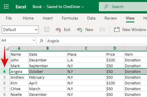
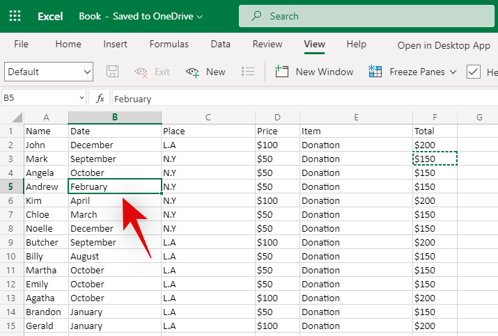
Open the involved Spreadsheet and discover the rows you want to freeze. Once discovered, click on and choose the row beneath your chosen rows by clicking on its quantity on the left aspect.

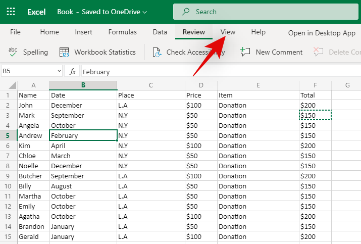
Once chosen, click on on ‘View’ on the prime of your display. 

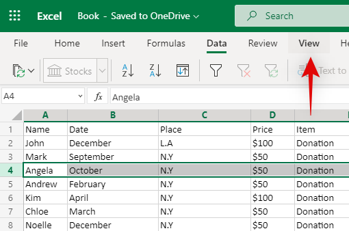
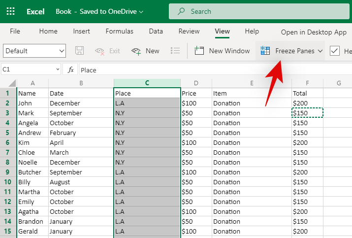
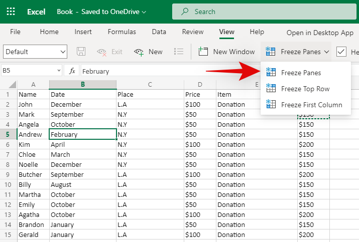
Now click on on ‘Freeze Panes’. 

Finally, choose ‘Freeze Panes’

And that’s it! All the rows above your chosen row will now be frozen and static in your display. They will all the time be seen no matter your place within the spreadsheet. 

Freeze Columns

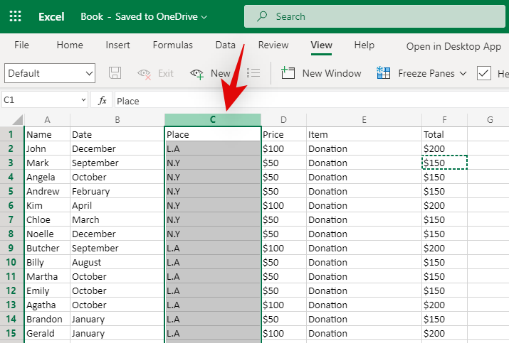
Open a spreadsheet and discover all of the columns you want to freeze. Now click on and choose your complete column to the suitable of your choice. 

Click on ‘View’ on the prime of your display. 

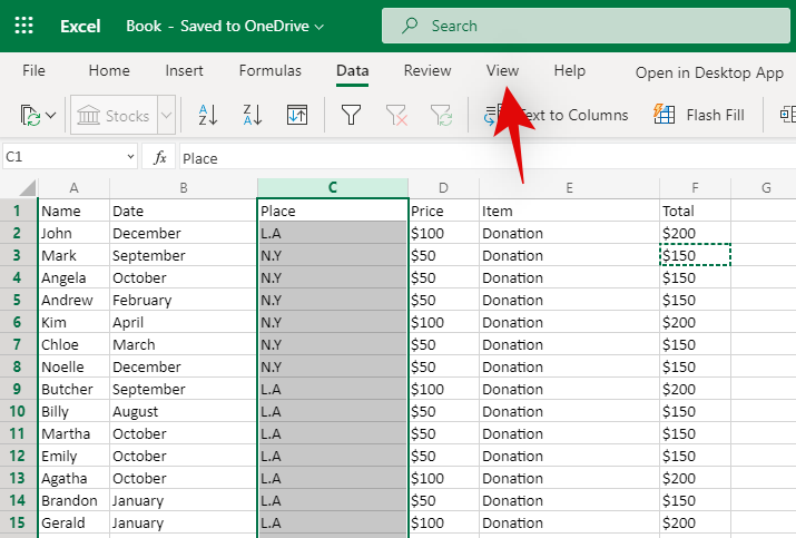
Now choose ‘Freeze Panes’. 

Click on ‘Freeze Panes’ to freeze all of the columns to the left of your choice. 

And that’s it! All the involved columns ought to now be frozen within the spreadsheet. They will stay static irrespective of how far you scroll horizontally.  

Freeze Rows & Columns

Find the rows and columns you want to freeze. Now choose the cell beneath the intersection of your choice. For instance, if you happen to want to choose columns A, B, and C, and row 1, 2, and three, then that you must choose cell D4. This can be the intersection level to your chosen rows and columns. 

Once chosen, click on on ‘View’ on the prime of your display. 

Now click on on ‘Freeze panes’. 

Click on ‘Freeze panes’ once more to freeze the rows and columns round your chosen cell. 

And that’s it! Your chosen rows and columns ought to now be frozen within the involved spreadsheet. 

I hope you have been simply in a position to freeze panes using the information above. If you may have any more questions, be happy to achieve out using the feedback part under.