How do I Highlight Duplicated Cells in Google Sheets

Are you looking for a technique to simply establish duplicate content material in your Google Sheets, significantly in massive datasets? Fortunately, there’s a simple approach. By adjusting a number of easy settings, you’ll be able to routinely spotlight duplicate content material/information in your chosen colour. Then, resolve whether or not to maintain or delete these duplicates. It’s fairly easy.

Here’s the step-by-step information to setting it up.

Highlight Duplicate Data in Google Sheets

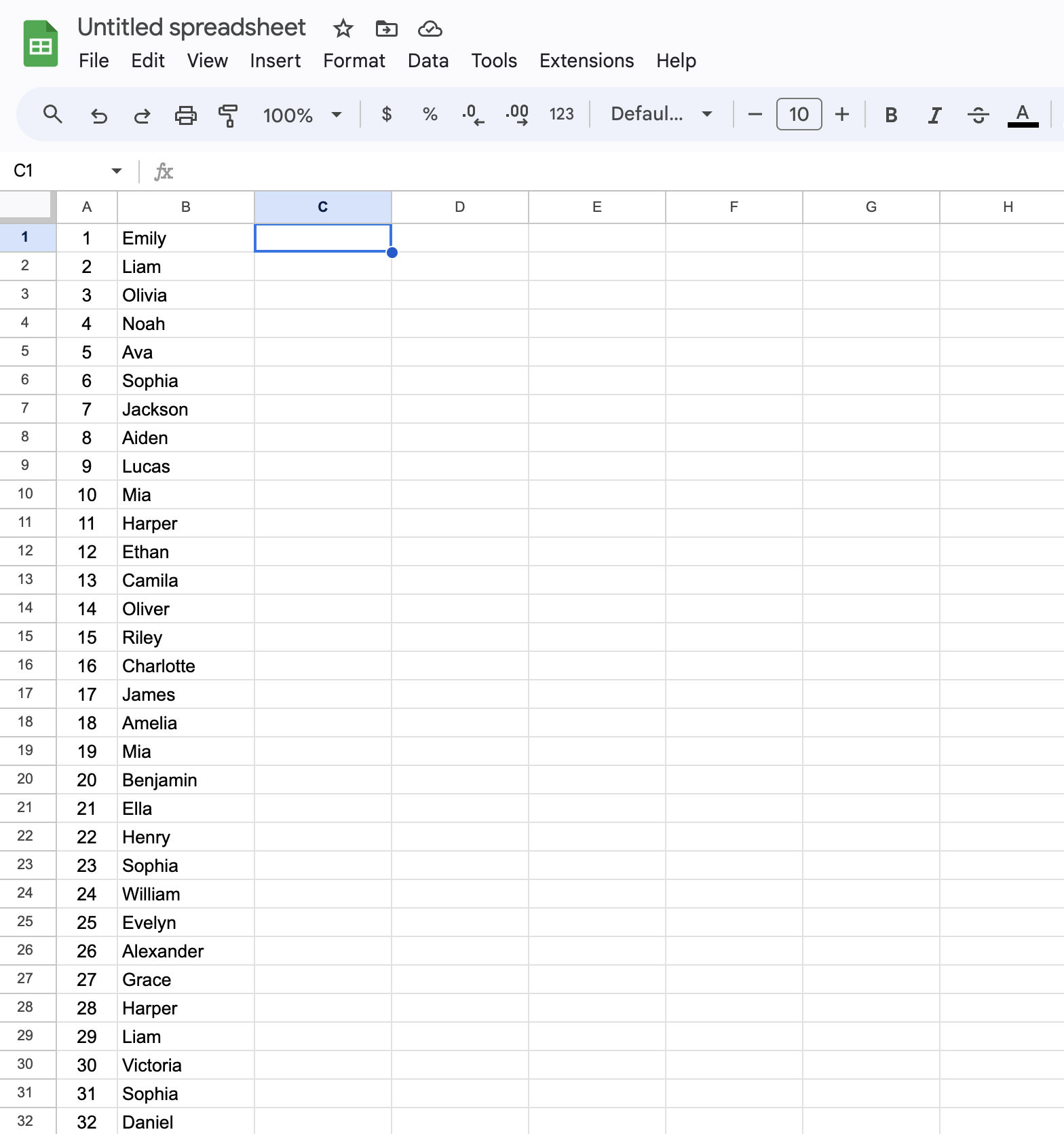
Suppose you have got a spreadsheet with a column of names in Column B and have to pinpoint the duplicates. Instead of manually scanning every title, Google Sheets can routinely spotlight them for you.

To spotlight duplicated information in Column B of Google Sheets, you’ll use Conditional Formatting with a customized method.

Here’s how you are able to do it:

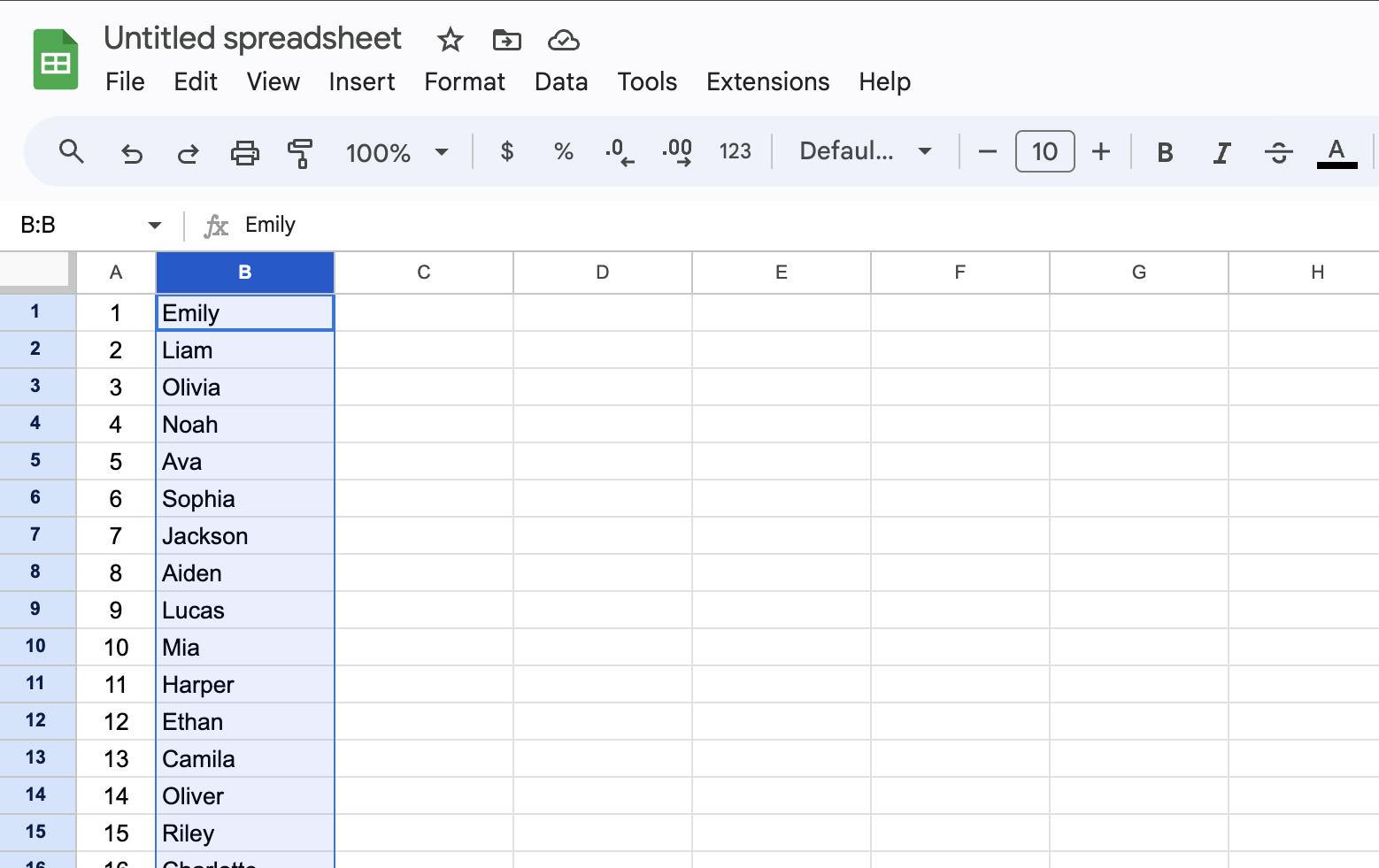
1. Select all the Column B by clicking on its header.



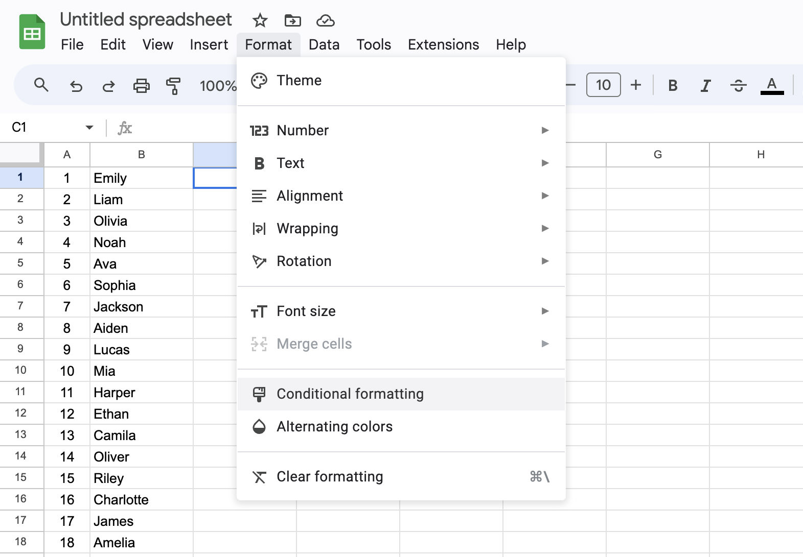
2. Navigate to the menu and choose Format > Conditional formatting.



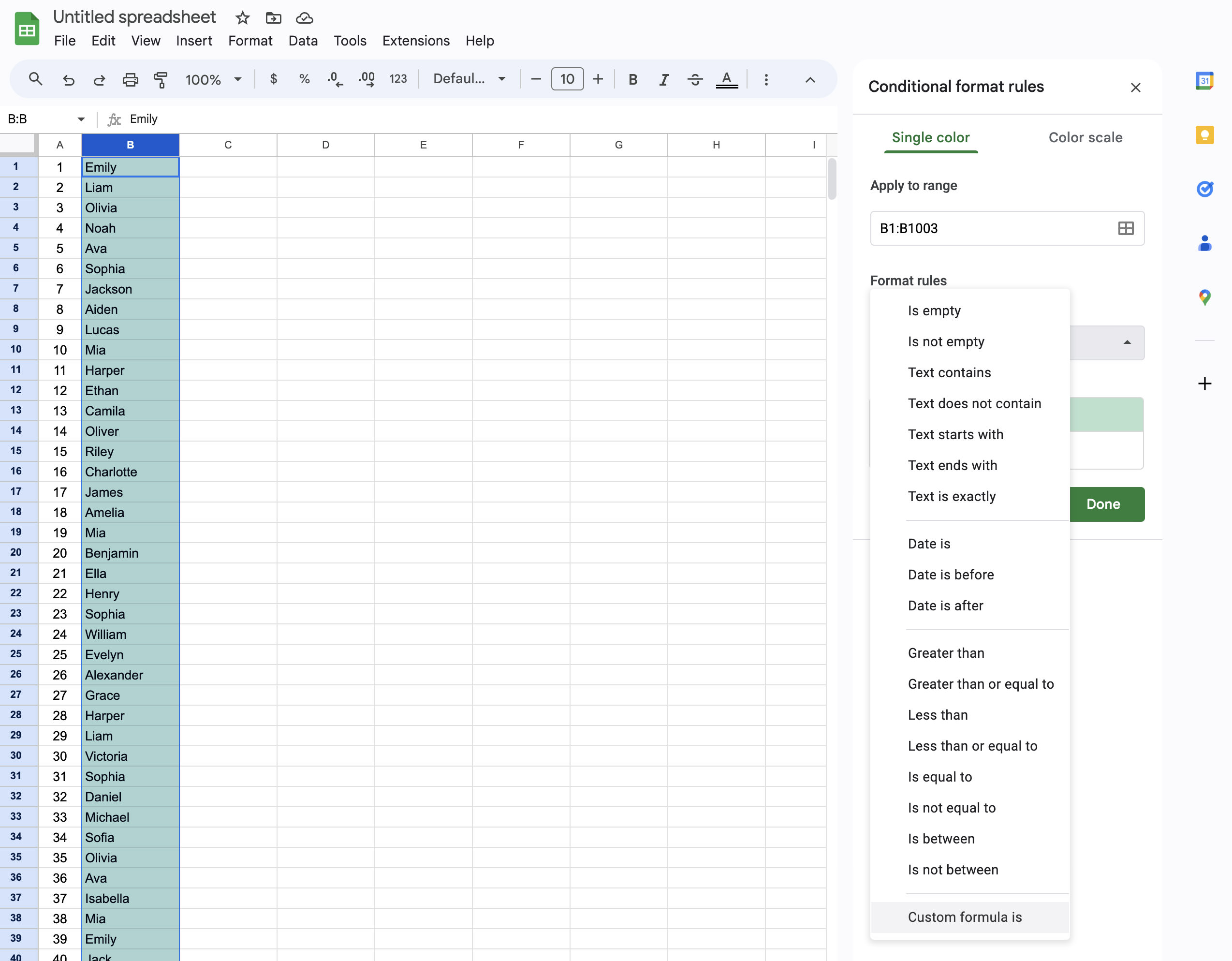
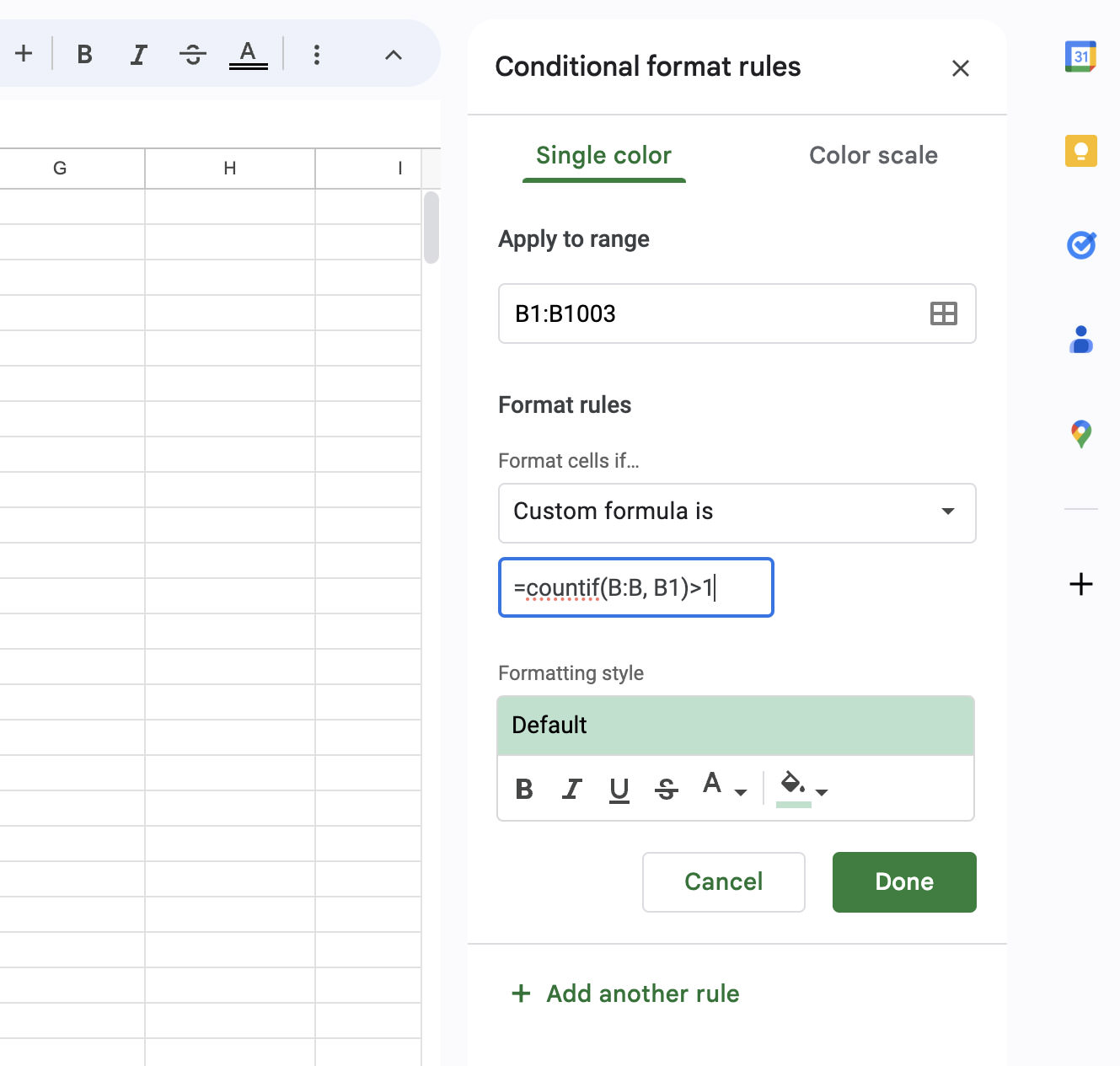
3. In the “Conditional format rules” sidebar on the proper, underneath the “Format cells if” dropdown, select “Custom formula is“.



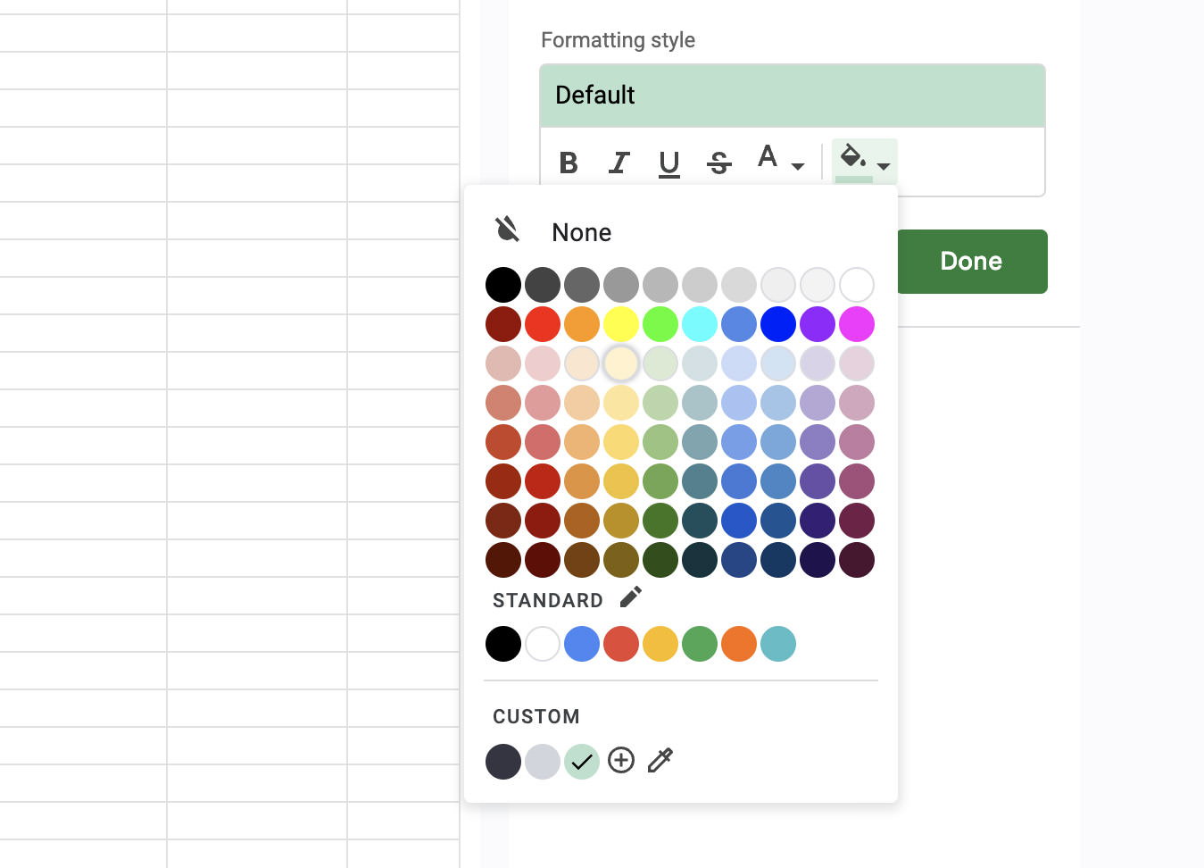
4. Input the next method: =countif(B:B, B1)>1. This method calculates how typically the worth in every cell of Column B seems in all the column. If a price seems greater than as soon as, the formatting you select can be utilized to these cells.



5. Select your required formatting type, like background colour, for the duplicate cells, after which click on “Done“.

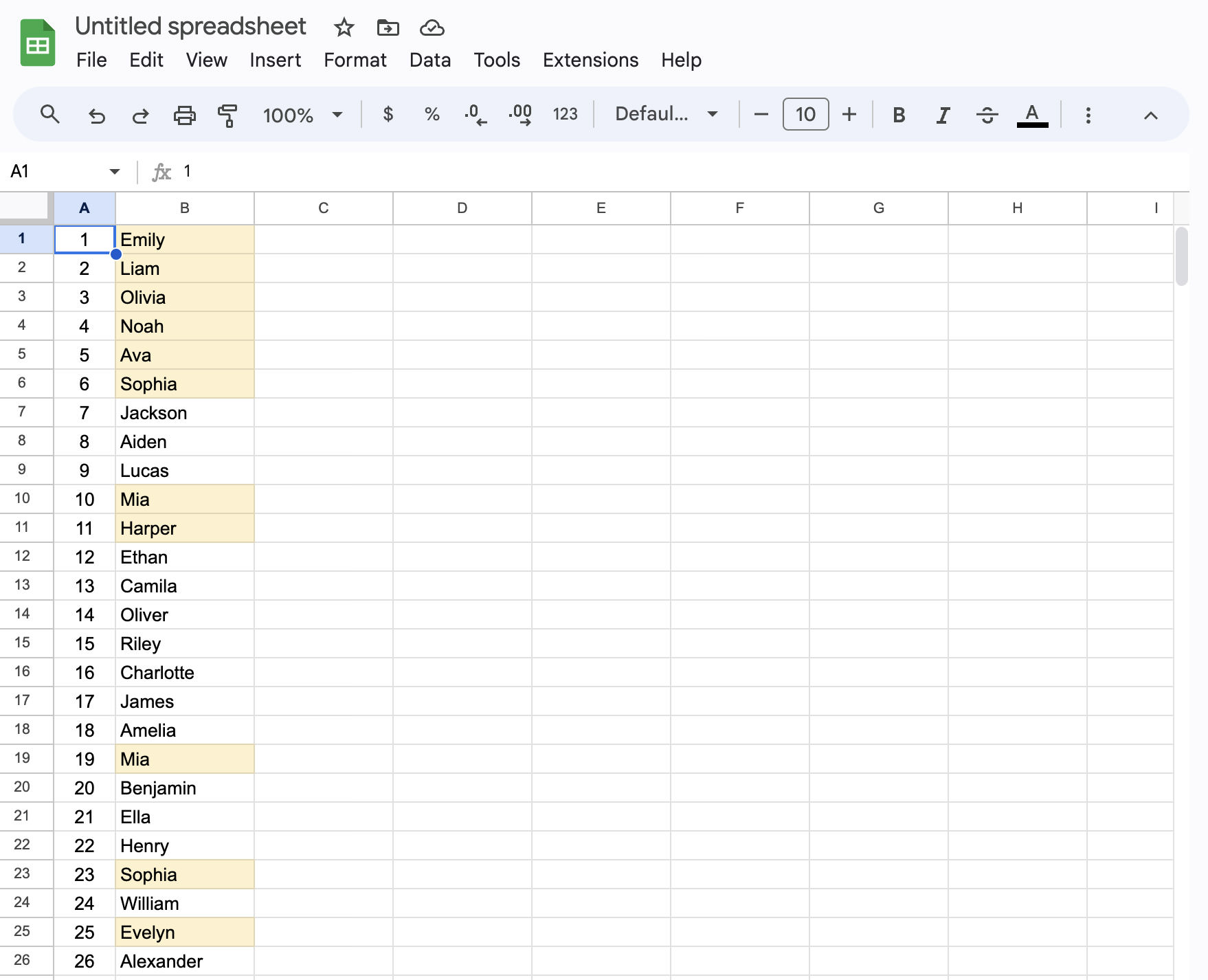
Once you’ve accomplished these steps, any cell in Column B with a price that seems greater than as soon as elsewhere within the column can be highlighted within the type you chose.

Another Simple Method…

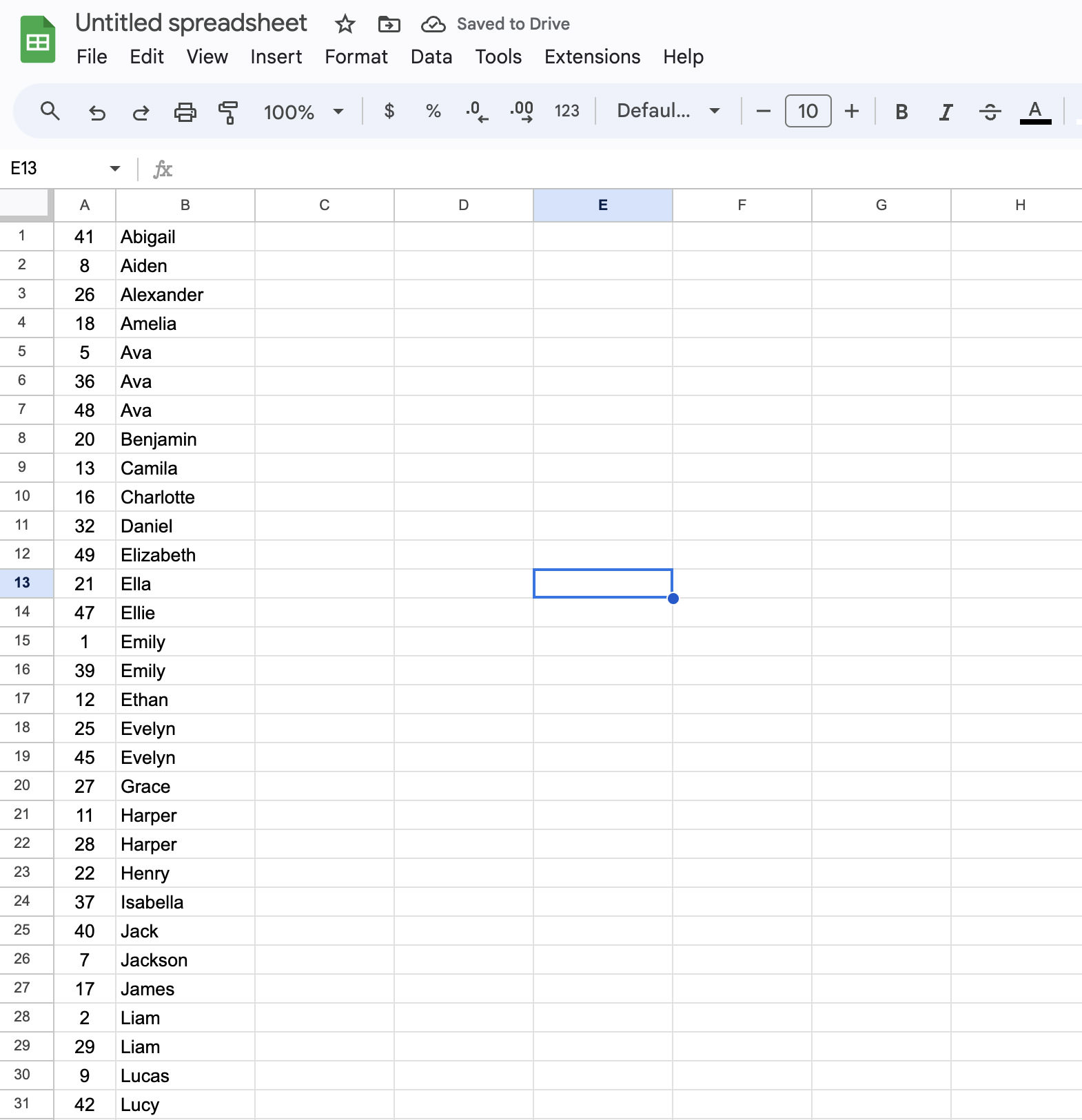
There’s yet one more easy methodology to identify duplicated information. Just hover over a cell in column B, click on on the arrow, and choose to kind all the column both A-Z or Z-A alphabetically.

Once sorted, any duplicated information, if current, can be grouped collectively. However, with out highlighting, this nonetheless requires a little bit of visible scanning to establish the duplicates.

Detect and Delete Duplicate Data

If your major purpose is just to detect and delete all duplicate information, with out the necessity for highlighting, observe these steps.

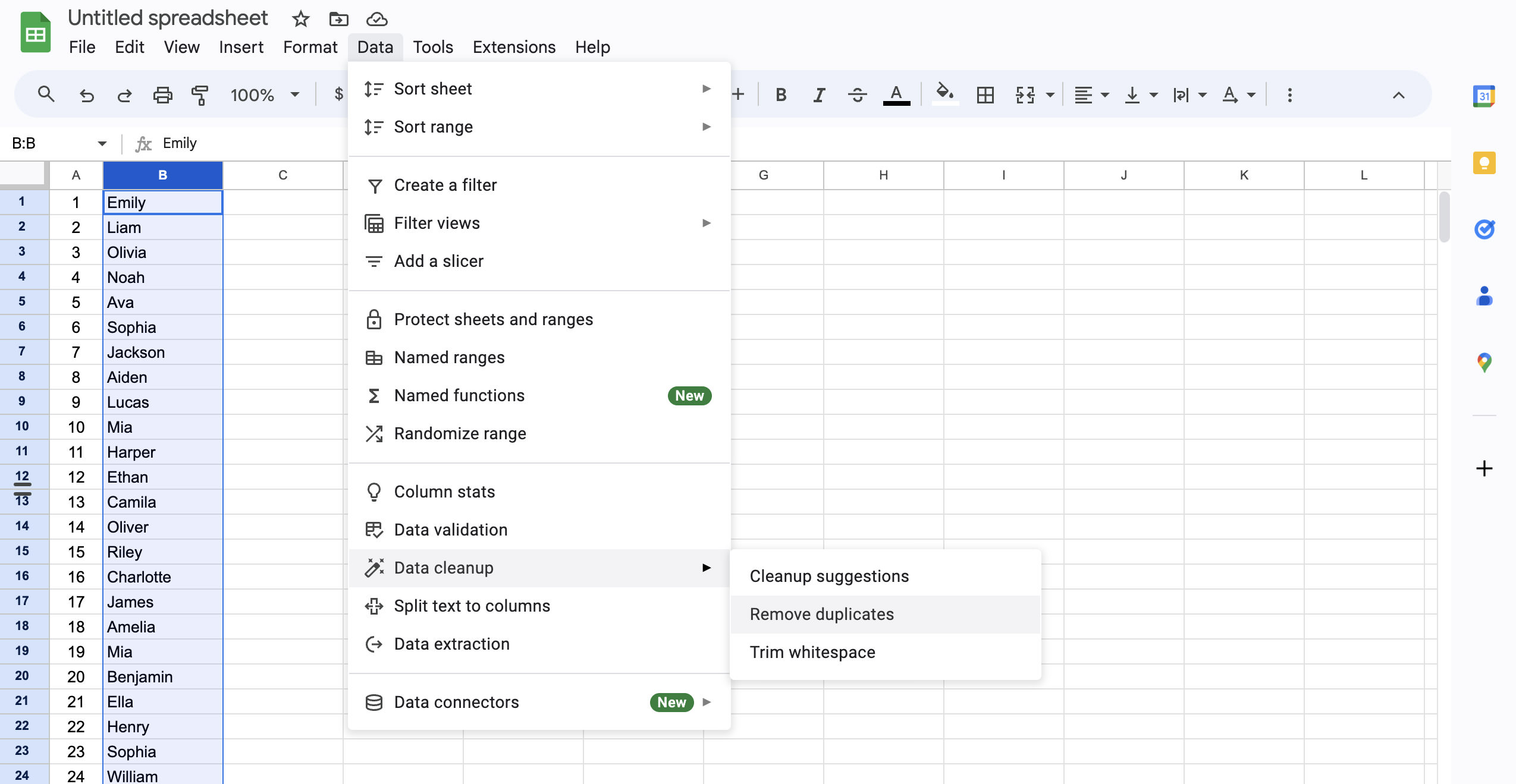
First, choose or spotlight Column B. Then, navigate via the menu: go to Data > Data cleanup > Remove duplicates.

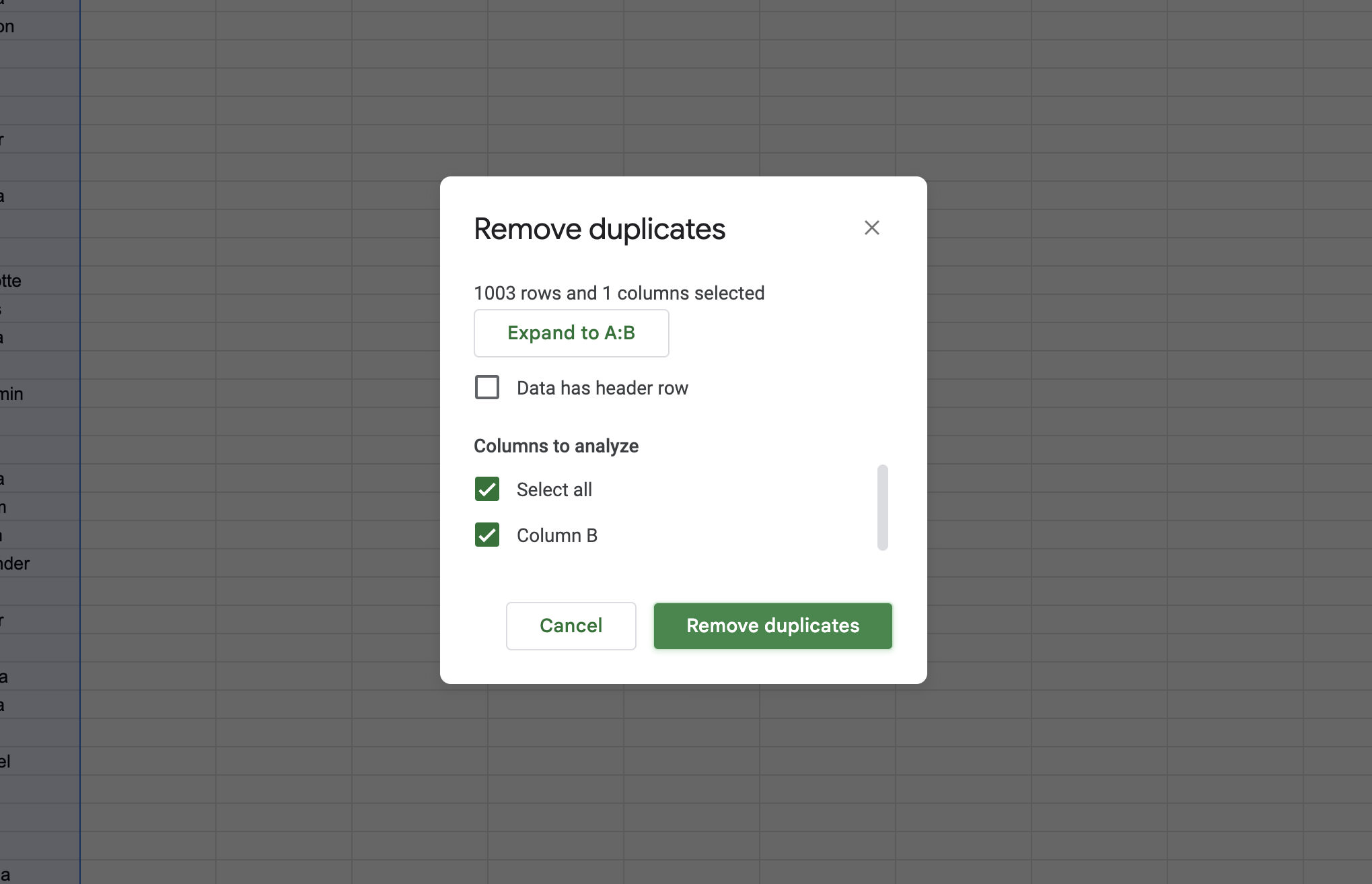
After that, click on on “Remove duplicates“.

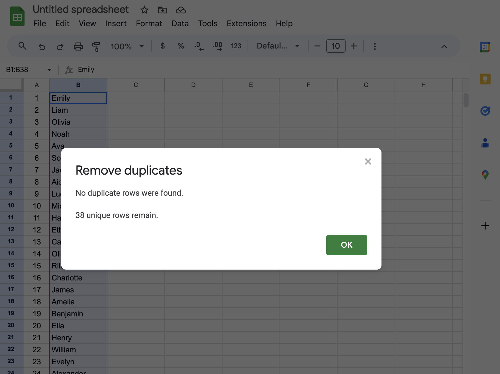
This motion will delete all duplicated information within the chosen column.